Please note that the data and information posted under the "Open Process" are for historical information only. They were preliminary information released in 1998-1999 as part of the SRES open process and for use in analysis to be contained in the IPCC Third Assessment Report (TAR). For final data (version 1.1) please go back to home page and follow the link.
IPCC Emission Scenario Database
Tsuneyuki Morita and Hae-Cheol Lee
The database can be obtained at http://www-cger.nies.go.jp/cger-e/db/ipcc.html. If other scenarios exist, the author’s will be pleased to receive details, and these will be included in any revisions of this database.
In order to identify future possible climate change impacts and to discover opportunities to stabilize the global climate, a very large number of scenarios have been prepared to be utilized in efforts to forecast greenhouse gas emissions. These scenarios were reviewed in the IPCC Special Report "Climate Change 1994" using several databases established by IIASA, PNL, NIES, IEW and EMF. However since 1994 new emission scenarios have been prepared, in response to changes in economic conditions and other events related to climate change, as well as new requests in the academic and policy fields. These emission scenarios are stored in computer files or in other media, but have not yet been systematically managed.
The IPCC Emission Scenario Database was established to manage the huge amount of data related to emission scenarios of greenhouse gases for the purpose to support activities on the IPCC Special Report on Emission Scenario (SRES) convened by Dr. Nebojsa Nakicenovic. For the database, a comprehensive collection of previous scenarios was attempted in order to conduct a new analysis to establish various story-lines and to establish a benchmark to be used to check the reliability and range of these scenarios. This document summarizes the database structure and the data collection for the database.
Database Structure
The main purpose behind the development of the new database is to make it easier to manage and utilize the cast amounts of data related to emission scenarios of greenhouse gases [GHGs], which include CO2, N2O, CH4, SOx and related gases (such as CO, NO2 and HFCs). The need to have such a database is a function of both the increasing number of emission scenarios- reflecting increasing political and research interests in this topic- and also of the need to be able to identify the strengths and weaknesses of current scenarios, allowing research to be focused on the most crucial or under-investigated areas.
These emission scenarios have mainly been quantified using computer simulation models, which in turn utilize a lot of assumptions on factors such as population growth, GDP growth, technology efficiency improvements, land-use changes, and the resource bases of energy. The assumptions used in incorporating these factors often differ between simulations, as does the actual factors represented in the simulations. As a result, the database was designed to manage the assumptions used to represent the various factors, as well as GHG emission scenarios.
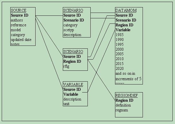
The database was designed on a relational database structure (using MS Access ‘97) because the data types incorporated were very diverse; the data itself represented many very large sized samples; and it was important to store the data using a structure which allowed one to also represent and store the relationships between different data types. The structure of the relational database is illustrated in the following diagram:

Each individual data entry is stored in the datamom. Using the relational structure, it is possible to call up data from within any of the four main fields (source ID, Scenario ID, region ID or variable) using a number of sub categories, each set of categories specific to the individual field. For example, the Source ID data entry field has the following subdivisions: source ID (an abbreviated model or organization name- multiple data sets are distinguished by year of publication); authors (name or organization name); reference (publication in which data is found); model (main simulation models); category (of simulation model, such as bottom up or top down, dynamic optimization of general equilibrium etc); updated date (of the most recent publication date; and notes (if any). The following table briefly summarizes the subdivisions in the other key fields:
|
Field name |
Subdivision (and brief description) |
||
|
Scenario |
Scenario ID (for reference scenario, or specific name of scenario, if one exists) |
Category (of scenario: non-intervention, intervention or uncertainty. Blank if scenario not identifiable. Non-intervention means a scenario with no reduction policies over carbon emission but which might include policies on other GHGs |
Description (of scenarios storyline and main assumptions) |
|
Region |
Region ID (many scenarios use different names for the same region. These are converted into one unique Region ID. The full country name is used for national studies) |
Definition (of each Region ID) |
|
|
Variable |
Description (of each variable for each source) |
Variable A common variable name is used for the same data item whose name varies between sources |
Unit |
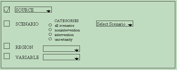
The database has the primary function of acting as a data storage tool, and an interface that will allow the user easy access to the data sets contained therein. In other words, it only provides data, and analyses are conducted using other tools such as spreadsheets. However, the relational structure of the database makes it possible to call up comparable data sets across the key fields, giving maximum flexibility in manipulation, extraction, and presentation of all the data in the database. Similarly, there is great flexibility in importing new data, or making a data set from the database using combinations of specific sources, specific scenarios (or categories), specific regions, and specific variables:

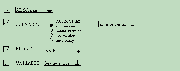
For example, using the extract function, one could set the following parameters: Extract all information on all scenarios in the AIM Japan source model, which examine the World sea level rise data. This would have the following Extraction screen:

It is also possible to make a data set using customized criteria. The database is thus very easy to use, even for a novice.
Future uses for the database include the possibility of putting it on the World Wide Web. Remote users will then be able to access the database and browse or retrieve a data set. Moreover, scenario results can be added to or modified by remote users. This will greatly reduce the workload needed to maintain the database and also improve data accuracy.
A sub-database, based on the original database, could be generated in parallel with the evaluation process of each sub group. Such subgroup databases could contain secondary data (like energy intensity, carbon intensity), some statistics (for example, the variation of carbon emissions by regions) or selected key variables for the evaluation process of each sub group.
Data Collection
The main sources of data used in compiling this report were: the International Energy Workshop Poll (of 1995, 1996, and 1997); Energy Modeling Forum (EMF-14 comparison studies) data; the previous database compiled for the IPCC Supplement Report, "Climate Change 1994" (Alcamo et al, 1995), which examined emission scenarios produced prior to 1994; and individuals emission scenarios collected by the authors.
The current database collection, covered in this report, includes the results of a total of 428 scenarios from 176 sources. These scenarios were mainly produced after 1994. Of the 428 scenarios, a total of 290 were global emission scenarios estimating GHG emission. Of these 290 global emission scenarios estimating greenhouse gas emissions [a full list of which is given in Appendix I], a total of 177 were non-intervention scenarios, and 113 intervention scenarios (assuming policies to mitigate climate changes).
Of the total of 428 scenarios, most focused on energy related CO2 emissions (372). Only three models estimated land-use related emissions: the ASF model for the IPCC 1992 scenarios; the IMAGE 2 model (at RIVM, the Netherlands); and the AIM model (at NIES, Japan). And very few scenarios considered global SO2 emissions.
The variable factors considered whilst collating scenario data, and the frequency such factors are found in the 428 scenarios (and thus stored in the SRES database), are listed in Tables in Appendix II. The regional disaggregations found amongst the 428 scenarios are listed in the following table:
Table 1 Regional disaggregations amongst global emission scenarios considering GHGs
|
Region ID |
Number of matching scenarios |
Region ID |
Number of matching scenarios |
|
World |
340 |
Extra |
12 |
|
OECD |
164 |
West Europe |
11 |
|
nonOECD |
158 |
DC |
7 |
|
China |
153 |
OSEAsia |
7 |
|
USA |
136 |
SubSAfrica |
6 |
|
FSU |
121 |
Annex 2 |
6 |
|
EEC |
85 |
Opacific |
6 |
|
Japan |
69 |
Poland |
5 |
|
FSU+EEU |
61 |
CSFR |
5 |
|
Annex 1 |
46 |
OPEC |
4 |
|
non Annex 1 |
46 |
United Kingdom |
4 |
|
Latin America |
42 |
LDC |
4 |
|
India |
36 |
EU 14 |
4 |
|
Africa |
34 |
EU 15 |
4 |
|
CPAsia |
32 |
EU 8 |
4 |
|
East Europe |
31 |
non OPEC DC |
3 |
|
ROW |
30 |
Hungary |
3 |
|
CANZ |
29 |
Switzerland |
3 |
|
Mexico and OPEC |
29 |
INDUS |
3 |
|
non OECD Annex 1 |
29 |
Asia Pacific |
2 |
|
Middle East |
27 |
Austria |
2 |
|
Oceania |
25 |
Brazil |
2 |
|
Canada |
24 |
DAE |
2 |
|
OECD Pacific |
23 |
ENX |
2 |
|
SouthAsia |
23 |
Germany |
2 |
|
OECD Europe |
22 |
Korea |
2 |
|
SEAsia |
16 |
Netherlands |
2 |
|
North America |
15 |
ROECD |
2 |
|
Europe |
12 |
ROW12 |
2 |
|
OECD West |
13 |
Sweden |
2 |
|
MEastNAfrica |
12 |
Nigeria |
2 |
|
East Asia |
12 |
19 other regions |
1 |
It should be noted that the breakdown of scenarios listed in this section represents the estimates generated from existing databases and the authors’ direct inquiries. The response rate for direct inquiries was not always high. If other scenarios exist, the author’s will be pleased to receive details, and these will be included in any revisions of this database.
Acknowledgements
The authors appreciate Dr. Arnulf Gruebler, Professor John Weyant, Professor Yuzuru Matsuoka, Dr. Eric Kreileman, Dr. Sruart R. Gaffin, Dr. Hugh M. Pitcher, Dr. Leo Schrattenholzer, and Professor Shunsuke Mori for their supports for data collection, and we also express our thankfulness to Mr. Ishii of Fuji Research Institute, Mr. Yoshinori Kobayashi and Miss Miki Yanagi for their tireless work for data conversion.